
Consulting & Research
Trusted by 100+
modellers and disaster experts
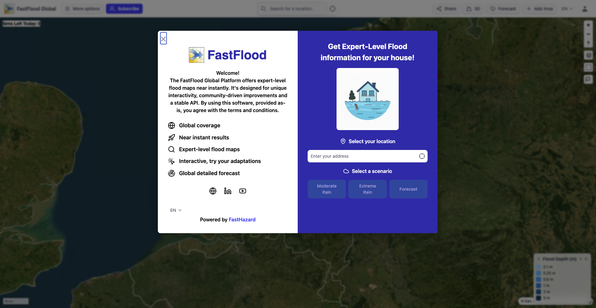
Our global community of users results in over 20,000 unique visitors every month
Try it out now


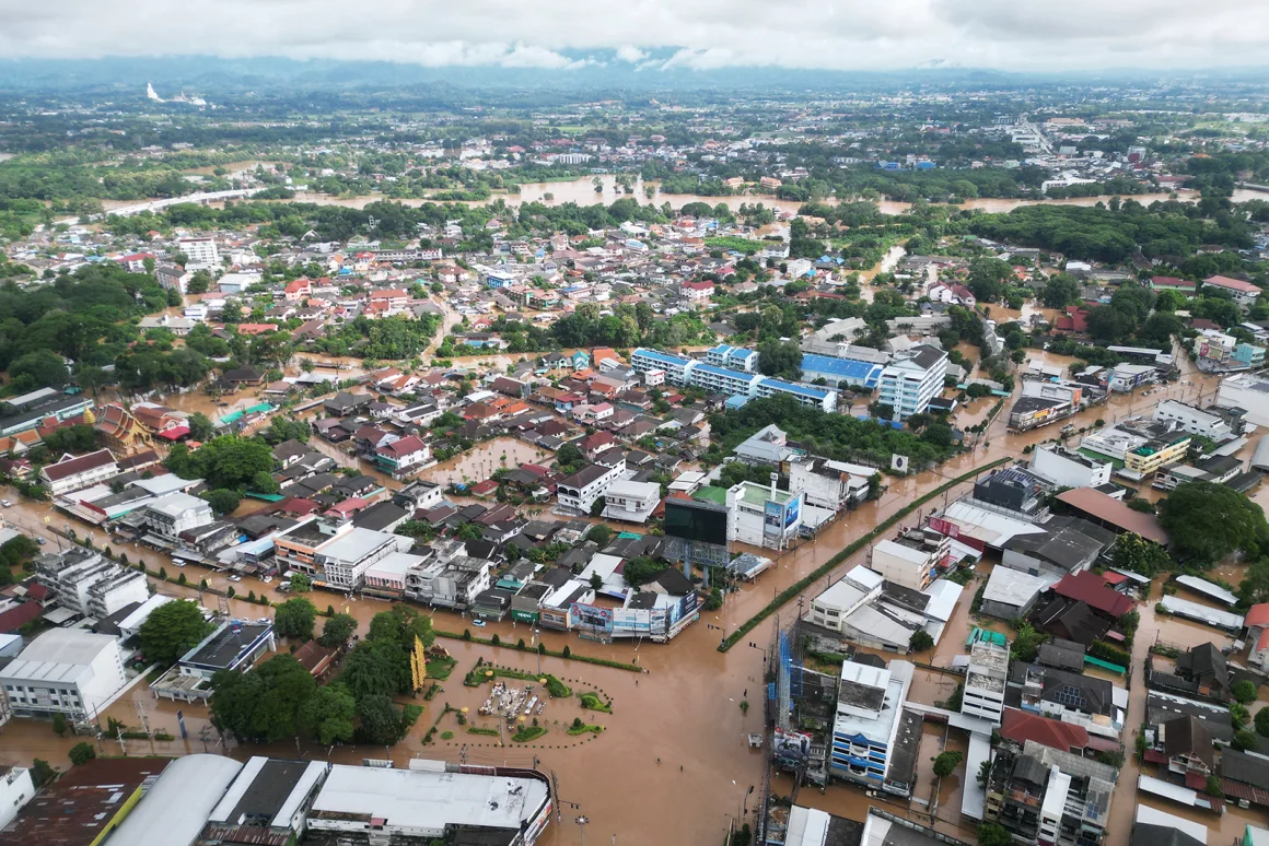
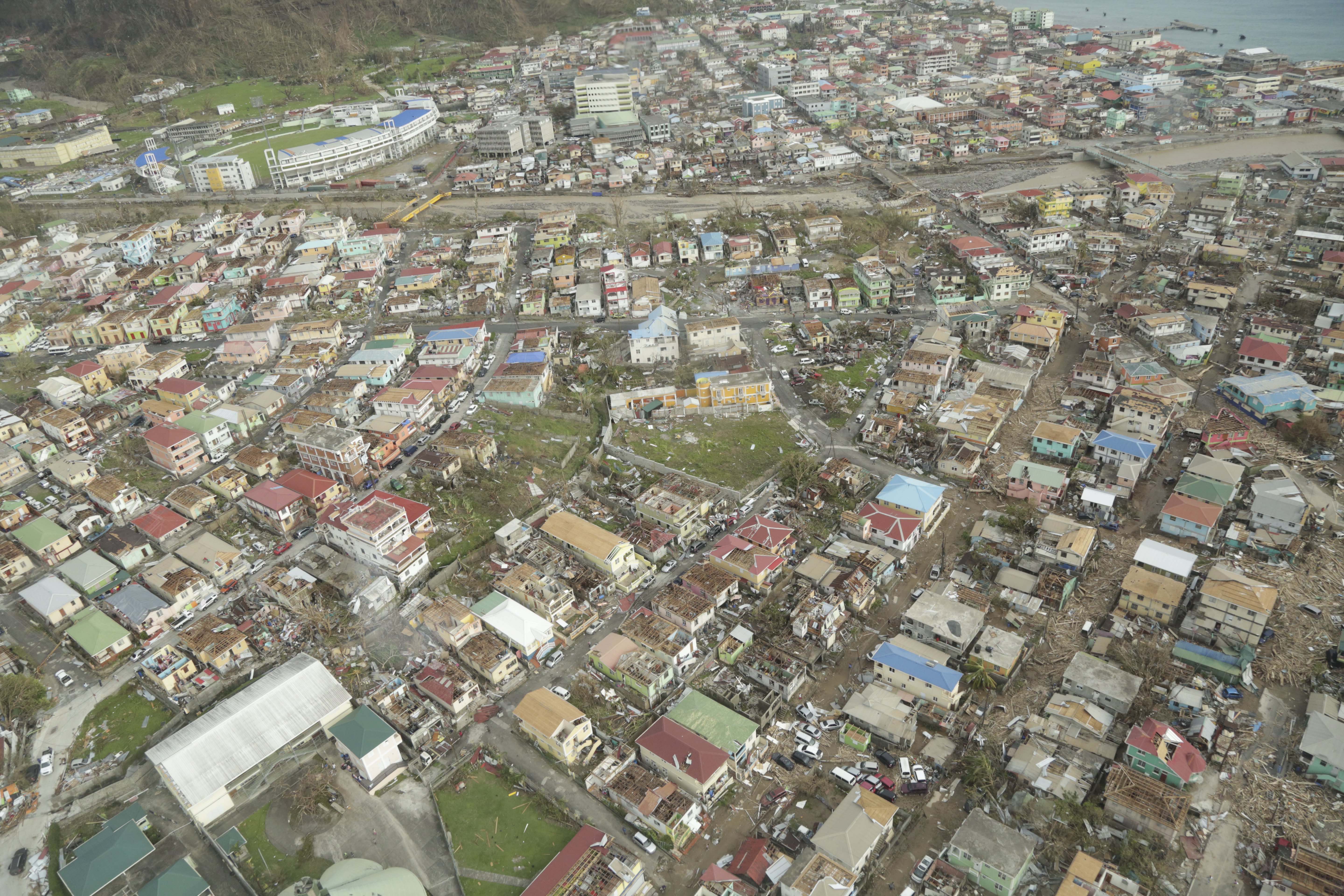
We conduct in-depth risk assessments for critical infrastructure, urban planning projects, and national adaptation strategies.
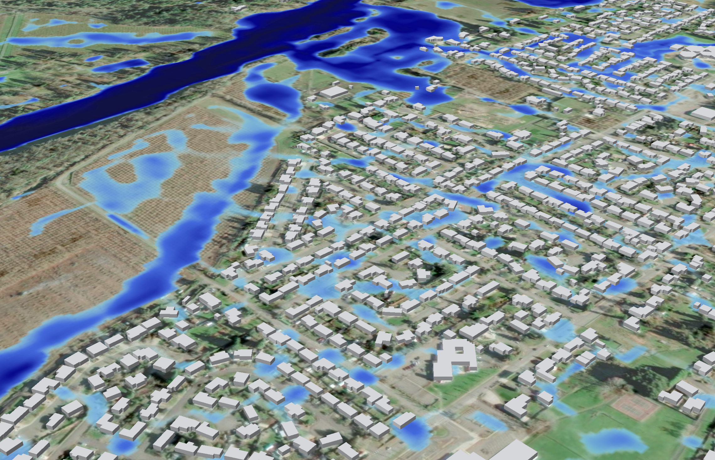
We work with national meteorological agencies and organizations to build and integrate state-of-the-art, automated early warning systems.
We help you design and test the effectiveness of adaptation measures, from large-scale levees to nature-based solutions, providing an evidence-based case for investment.
Our global community of users results in over 20,000 unique visitors every month
Try it out now
From academic research to enterprise-level infrastructure planning, find the Fast Flood plan that fits your needs. Start simulating for free today.
Pricing per Seat